This page was generated by
nbsphinx from
docs/notebooks/analysis/fit_functions.ipynb.
Interactive online version:
![]() .
.
Fit Functions
Fit functions are a set of callable classes designed to aid in fitting analytical functions to data. A fit function class combines the following functionality:
An analytical function that is callable with given parameters or fitted parameters.
Curve fitting functionality (usually SciPy’s curve_fit() or linregress()), which stores the fit statistics and parameters into the class. This makes the function easily callable with the fitted parameters.
Error propagation calculations.
A root solver that returns either the known analytical solutions or uses SciPy’s fsolve() to calculate the roots.
[1]:
%matplotlib inline

import matplotlib.pyplot as plt
import numpy as np

from plasmapy.analysis import fit_functions as ffuncs

plt.rcParams["figure.figsize"] = [10.5, 0.56 * 10.5]
Contents:
Fit function basics
There is an ever expanding collection of fit functions, but this notebook will use ExponentialPlusLinear as an example.
A fit function class has no required arguments at time of instantiation.
[2]:
# basic instantiation
explin = ffuncs.ExponentialPlusLinear()

# fit parameters are not set yet
(explin.params, explin.param_errors)
[2]:
(None, None)
Each fit parameter is given a name.
[3]:
[3]:
('a', 'alpha', 'm', 'b')
These names are used throughout the fit function’s documentation, as well as in its __repr__, __str__, and latex_str methods.
[4]:
(explin, explin.__str__(), explin.latex_str)
[4]:
(f(x) = a exp(alpha x) + m x + b <class 'plasmapy.analysis.fit_functions.ExponentialPlusLinear'>,
 'f(x) = a exp(alpha x) + m x + b',
 'a \\, \\exp(\\alpha x) + m x + b')
Fitting to data
Fit functions provide the curve_fit() method to fit the analytical function to a set of \((x, y)\) data. This is typically done with SciPy’s curve_fit() function, but fitting is done with SciPy’s linregress() for the Linear fit function.
Let’s generate some noisy data to fit to…
[5]:
params = (5.0, 0.1, -0.5, -8.0)  # (a, alpha, m, b)
xdata = np.linspace(-20, 15, num=100)
ydata = explin.func(xdata, *params) + np.random.normal(0.0, 0.6, xdata.size)

plt.plot(xdata, ydata)
plt.xlabel("X", fontsize=14)
plt.ylabel("Y", fontsize=14)
[5]:
Text(0, 0.5, 'Y')

The fit function curve_fit() shares the same signature as SciPy’s curve_fit(), so any **kwargs will be passed on. By default, only the \((x, y)\) values are needed.
[6]:
explin.curve_fit(xdata, ydata)
Getting fit results
After fitting, the fitted parameters, uncertainties, and coefficient of determination, or \(r^2\), values can be retrieved through their respective properties, params, parame_errors, and rsq.
[7]:
(explin.params, explin.params.a, explin.params.alpha)
[7]:
(FitParamTuple(a=4.976242026810416, alpha=0.09977503326350426, m=-0.4888017144781502, b=-7.895046380079913),
 4.976242026810416,
 0.09977503326350426)
[8]:
(explin.param_errors, explin.param_errors.a, explin.param_errors.alpha)
[8]:
(FitParamTuple(a=1.0550988537502097, alpha=0.009342702129421825, m=0.04728639153131081, b=1.0795094663666458),
 1.0550988537502097,
 0.009342702129421825)
[9]:
[9]:
np.float64(0.9461145330973174)
Fit function is callable
Now that parameters are set, the fit function is callable.
[10]:
explin(0)
[10]:
np.float64(-2.918804353269497)
Associated errors can also be generated.
[11]:
y, y_err = explin(np.linspace(-1, 1, num=10), reterr=True)
(y, y_err)
[11]:
(array([-2.90254161, -2.91019182, -2.91557824, -2.91865012, -2.91935557,
        -2.91764154, -2.91345377, -2.9067368 , -2.89743394, -2.88548721]),
 array([1.44263505, 1.45636776, 1.47072844, 1.48573478, 1.50140492,
        1.51775746, 1.53481148, 1.55258654, 1.57110273, 1.5903806 ]))
Known uncertainties in \(x\) can be specified too.
[12]:
y, y_err = explin(np.linspace(-1, 1, num=10), reterr=True, x_err=0.1)
(y, y_err)
[12]:
(array([-2.90254161, -2.91019182, -2.91557824, -2.91865012, -2.91935557,
        -2.91764154, -2.91345377, -2.9067368 , -2.89743394, -2.88548721]),
 array([1.44264045, 1.45637072, 1.47072968, 1.48573503, 1.50140494,
        1.51775804, 1.53481343, 1.55259072, 1.57110999, 1.59039184]))
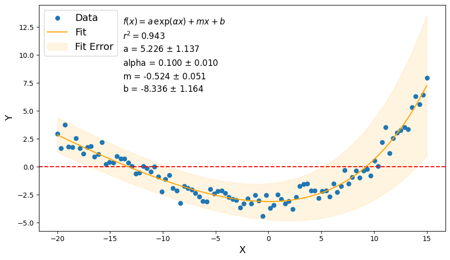
Plotting results
[13]:
# plot original data
plt.plot(xdata, ydata, marker="o", linestyle=" ", label="Data")
ax = plt.gca()
ax.set_xlabel("X", fontsize=14)
ax.set_ylabel("Y", fontsize=14)

ax.axhline(0.0, color="r", linestyle="--")

# plot fitted curve + error
yfit, yfit_err = explin(xdata, reterr=True)
ax.plot(xdata, yfit, color="orange", label="Fit")
ax.fill_between(
    xdata,
    yfit + yfit_err,
    yfit - yfit_err,
    color="orange",
    alpha=0.12,
    zorder=0,
    label="Fit Error",
)

# plot annotations
plt.legend(fontsize=14, loc="upper left")

txt = f"$f(x) = {explin.latex_str}$\n$r^2 = {explin.rsq:.3f}$\n"
for name, param, err in zip(
    explin.param_names, explin.params, explin.param_errors, strict=False
):
    txt += f"{name} = {param:.3f} $\\pm$ {err:.3f}\n"
txt_loc = [-13.0, ax.get_ylim()[1]]
txt_loc = ax.transAxes.inverted().transform(ax.transData.transform(txt_loc))
txt_loc[0] -= 0.02
txt_loc[1] -= 0.05
ax.text(
    txt_loc[0],
    txt_loc[1],
    txt,
    fontsize="large",
    transform=ax.transAxes,
    va="top",
    linespacing=1.5,
)
[13]:
Text(0.20727272727272733, 0.95, '$f(x) = a \\, \\exp(\\alpha x) + m x + b$\n$r^2 = 0.946$\na = 4.976 $\\pm$ 1.055\nalpha = 0.100 $\\pm$ 0.009\nm = -0.489 $\\pm$ 0.047\nb = -7.895 $\\pm$ 1.080\n')
Root solving
An exponential plus a linear offset has no analytical solutions for its roots, except for a few specific cases. To get around this, ExponentialPlusLinear().root_solve() uses SciPy’s fsolve() to calculate it’s roots. If a fit function has analytical solutions to its roots (e.g. Linear().root_solve()), then the method is overridden with the known solution.
[14]:
root, err = explin.root_solve(-15.0)
(root, err)
[14]:
(np.float64(-13.506274243259888), nan)
Let’s use Linear().root_solve() as an example for a known solution.
[15]:
lin = ffuncs.Linear(params=(1.0, -5.0), param_errors=(0.1, 0.1))
root, err = lin.root_solve()
(root, err)
[15]:
(5.0, np.float64(0.5099019513592785))